Contents
Ejercicio 1
x=[10;20;40;60;80];
y=[x,log(x)];

fprintf('\n Numero Natural \t log\n')
fprintf('\t%4i\t\t%8.5f\n',y')
 Numero Natural 	 log
	  10		 2.30259
	  20		 2.99573
	  40		 3.68888
	  60		 4.09434
	  80		 4.38203
Ejercicio 2
A = [4 -2 -10; 2 10 -12; -4 -6 16];
B = [-10; 32; -16];
X=A\B
X =

    2.0000
    4.0000
    1.0000
Ejercicio 3
A=[4 -2 -10;2 10 -12;-4 -6 16];
b=[-10 32 -16]';
[L U]=lu(A)
C=L*U
X=inv(U)*inv(L)*b
L =

    1.0000         0         0
    0.5000    1.0000         0
   -1.0000   -0.7273    1.0000


U =

    4.0000   -2.0000  -10.0000
         0   11.0000   -7.0000
         0         0    0.9091


C =

     4    -2   -10
     2    10   -12
    -4    -6    16


X =

     2
     4
     1
Ejercicio 4
A = [0 1 -1; -6 -11 6; -6 -11 5];
[V, D] = eig(A)
V =

    0.7071   -0.2182   -0.0921
    0.0000   -0.4364   -0.5523
    0.7071   -0.8729   -0.8285


D =

   -1.0000         0         0
         0   -2.0000         0
         0         0   -3.0000
Ejercicio 5
R = [1.5-2i, -0.35+1.2i; -0.35+1.2i, 0.9-1.6i];
I = [30+40i; 20+15i];
V = R\I
S = V.*conj(I)
V =

   3.5902 +35.0928i
   6.0155 +36.2212i


S =

   1.0e+03 *

   1.5114 + 0.9092i
   0.6636 + 0.6342i
Ejercicio 6
hanoi(5,'a','b','c')
mover disco 1 de a a c
mover disco 2 de a a b
mover disco 1 de c a b
mover disco 3 de a a c
mover disco 1 de b a a
mover disco 2 de b a c
mover disco 1 de a a c
mover disco 4 de a a b
mover disco 1 de c a b
mover disco 2 de c a a
mover disco 1 de b a a
mover disco 3 de c a b
mover disco 1 de a a c
mover disco 2 de a a b
mover disco 1 de c a b
mover disco 5 de a a c
mover disco 1 de b a a
mover disco 2 de b a c
mover disco 1 de a a c
mover disco 3 de b a a
mover disco 1 de c a b
mover disco 2 de c a a
mover disco 1 de b a a
mover disco 4 de b a c
mover disco 1 de a a c
mover disco 2 de a a b
mover disco 1 de c a b
mover disco 3 de a a c
mover disco 1 de b a a
mover disco 2 de b a c
mover disco 1 de a a c
Ejercicio 7
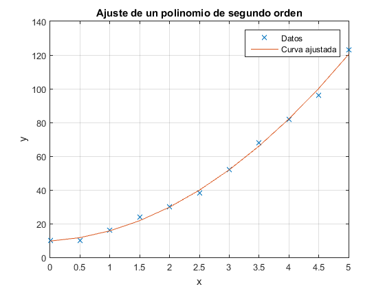
x = [0 0.5 1 1.5 2 2.5 3 3.5 4 4.5 5];
y = [10 10 16 24 30 38 52 68 82 96 123];
P = polyfit(x,y,2)
yc = polyval(P,x)
figure(1)
plot(x,y,'x',x,yc);
title('Ajuste de un polinomio de segundo orden');
xlabel('x'); ylabel('y');legend('Datos','Curva ajustada');grid;
P =

    4.0233    2.0107    9.6783


yc =

  Columns 1 through 7

    9.6783   11.6895   15.7124   21.7469   29.7930   39.8508   51.9203

  Columns 8 through 11

   66.0014   82.0942  100.1986  120.3147
Ejercicio 8
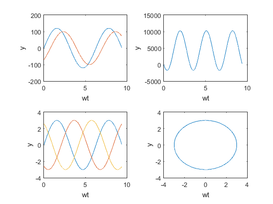
wt = 0:0.05:3*pi;
v = 120.*sin(wt);
k = 100.*sin(wt-pi/4);
figure(2)
subplot(2,2,1);
plot(wt,v,wt,k);xlabel('wt'); ylabel('y');
subplot(2,2,2);
p = v.*k;
plot(wt,p);xlabel('wt'); ylabel('y');
subplot(2,2,3);
Fm = 3;
fa = Fm.*sin(wt);
fb = Fm.*sin(wt-(2*pi)/3);
fc = Fm.*sin(wt-(4*pi)/3);
plot(wt,fa,wt,fb,wt,fc);xlabel('wt'); ylabel('y');
subplot(2,2,4);
fR=3;
plot(-fR.*cos(wt),fR.*sin(wt));xlabel('wt'); ylabel('y');
Ejercicio 9
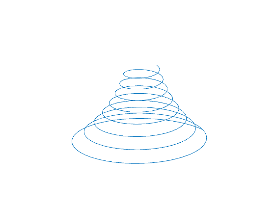
t=0:0.1:16*pi;
X=exp(-0.03*t).*cos(t);
Y=exp(-0.03*t).*sin(t);
Z=t;
subplot(1,1,1)
plot3(X,Y,Z), axis off
Ejercicio 11
f=[1 0 -35 50 24];
r=roots(f)
r =

   -6.4910
    4.8706
    2.0000
   -0.3796
Ejercicio 12
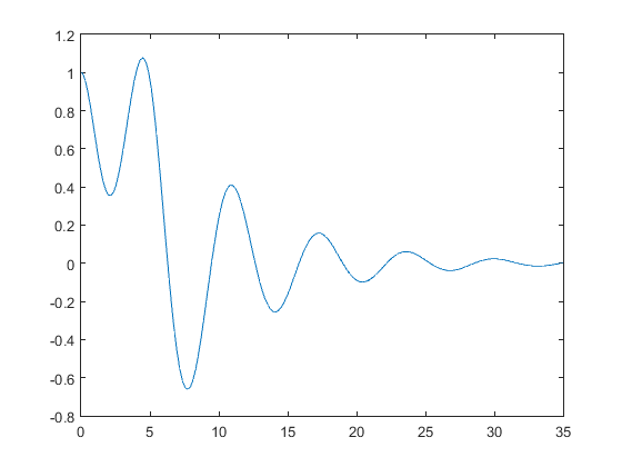
[t, yy] = ode45(@HalfSine, [0 35], [1 0], [ ], 0.15);
figure(3)
plot(t, yy(:,1))
Ejercicio 13a)
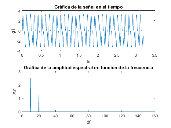
k = 5; m = 10; fo = 10; Bo = 2.5; N = 2^m; T = 2^k/fo;
ts = (0:N-1)*T/N; df = (0:N/2-1)/T;
g1 = Bo*sin(2*pi*fo*ts)+Bo/2*sin(2*pi*fo*2*ts);
An = abs(fft(g1, N))/N;
figure(4)
subplot(2,1,1)
plot(ts,g1);title('Gráfica de la señal en el tiempo');
xlabel('ts'); ylabel('g1');
subplot(2,1,2)
plot(df,2*An(1:N/2));title('Gráfica de la amplitud espectral en función de la frecuencia');
xlabel('df'); ylabel('An');
Ejercicio 13b)
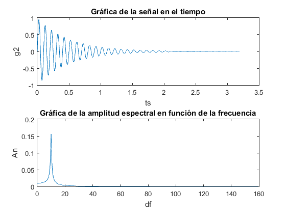
k = 5; m = 10; fo = 10; Bo = 2.5; N = 2^m; T = 2^k/fo;
ts = (0:N-1)*T/N; df = (0:N/2-1)/T;
g2 = exp(-2*ts).*sin(2*pi*fo*ts);
An = abs(fft(g2, N))/N;
figure(5)
subplot(2,1,1)
plot(ts,g2),title('Gráfica de la señal en el tiempo');
xlabel('ts'), ylabel('g2');
subplot(2,1,2)
plot(df,2*An(1:N/2)),title('Gráfica de la amplitud espectral en función de la frecuencia');
xlabel('df'), ylabel('An');
Ejercicio 13c)
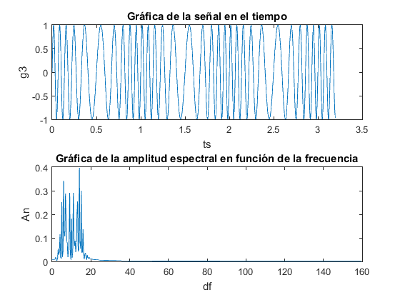
k = 5; m = 10; fo = 10; Bo = 2.5; N = 2^m; T = 2^k/fo;
ts = (0:N-1)*T/N; df = (0:N/2-1)/T;
g3 = sin(2*pi*fo*ts+5*sin(2*pi*(fo/10)*ts));
An = abs(fft(g3, N))/N;
figure(6)
subplot(2,1,1)
plot(ts,g3);title('Gráfica de la señal en el tiempo');
xlabel('ts'); ylabel('g3');
subplot(2,1,2)
plot(df,2*An(1:N/2));title('Gráfica de la amplitud espectral en función de la frecuencia');
xlabel('df'); ylabel('An');
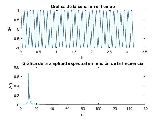
Ejercicio 13d)
k = 5; m = 10; fo = 10; Bo = 2.5; N = 2^m; T = 2^k/fo;
ts = (0:N-1)*T/N; df = (0:N/2-1)/T;
g4 = sin(2*pi*fo*ts-5*exp(-2*ts));
An = abs(fft(g4, N))/N;
figure(7)
subplot(2,1,1)
plot(ts,g4);title('Gráfica de la señal en el tiempo');
xlabel('ts'); ylabel('g4');
subplot(2,1,2)
plot(df,2*An(1:N/2));title('Gráfica de la amplitud espectral en función de la frecuencia');
xlabel('df'); ylabel('An');
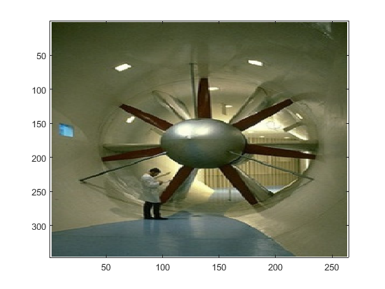
Ejercicio 14
figure(8)
v = imread('WindTunnel.jpg');
image(v)
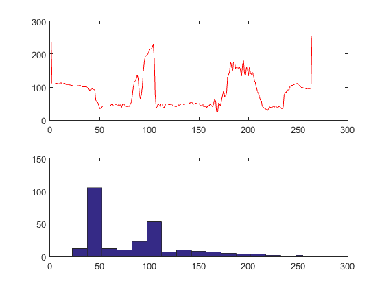
figure(9)
row = 200;
red = v(row, :, 1);
gr = v(row, :, 2);
bl = v(row, :, 3);
subplot(2,1,1)
plot(red, 'r');
subplot(2,1,2)
hist(red,0:15:255)
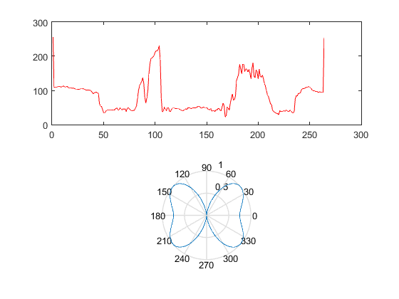
Ejercicio 15
theta = linspace(-pi, pi, 300);
p = abs(besselj(2, -4*cos(theta)));
polar(theta, p/max(p))